STEP 1: Obtaining/Cleaning the data
Turtle Games provided a single dataset combining customer demographics (age, gender, education, remuneration), spending score, loyalty points, and review text. Two constant fields (language, platform) were dropped immediately, as they carried no discriminatory value; columns were renamed for consistency, and the data were checked for missing values and outliers using pandas before proceeding, with no material issues found.

STEP 2: Initial regression analysis
Regression was implemented in scikit-learn using LinearRegression, first fitted individually to age, remuneration and spending (isolating each predictor’s standalone R-squared) before combining all three into a multiple linear regression. A train_test_split (80/20, fixed random_state for reproducibility) was used throughout to guard against overfitting. The same model was rebuilt independently in R, which allowed two extra checks: one for multicollinearity (whether the predictor variables overlap too much with each other, using car::vif()), and one for distributional assumptions (whether the data behaves normally enough for linear regression to be valid, using shapiro.test() and e1071::skewness()/kurtosis()). Performing the analysis in two languages provided an informal crossvalidation: consistent coefficients across two independent implementations increased confidence beyond what either language alone would justify.

STEP 3: Decision Tree Regressor
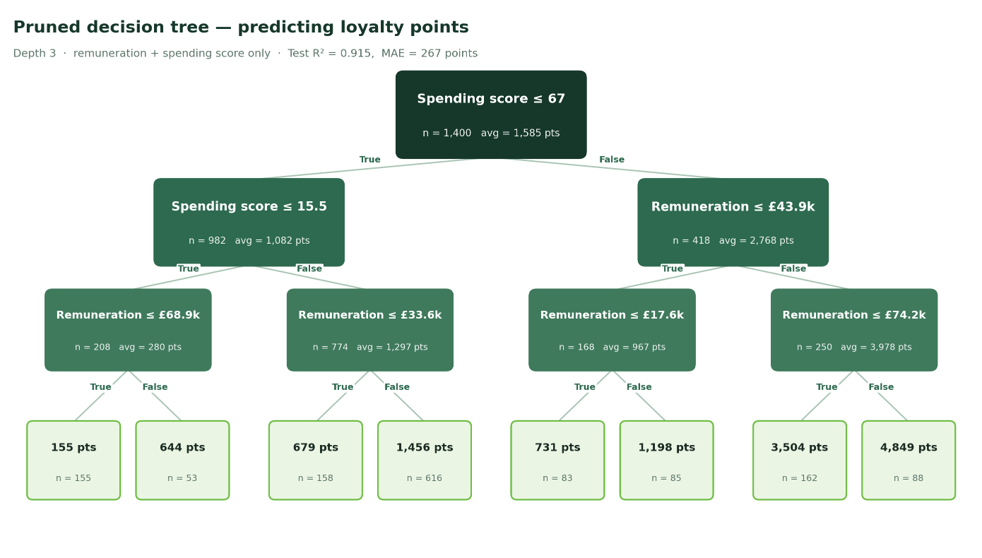
A DecisionTreeRegressor was grown separately, since regression coefficients, while precise, are not something a marketing team can operationalise directly. An unconstrained tree (max_depth=10) was fitted first and rejected on the basis of a near-perfect training R-squared (0.997), a clear overfitting signal; a depth-versus-accuracy sweep (1-20) and feature_importances_ ranking were then used to prune deliberately, removing education, product type and gender (negligible importance) and finally age, arriving at a max_depth=3 tree using only remuneration and spending, with min_samples_split and min_samples_leaf constraints added to prevent tiny, unstable leaf nodes. For prediction, the depth-3 decision tree (test R-squared=0.915, MAE=267 points) is recommended for operational use over the full regression model, since its small accuracy loss is outweighed by the interpretability gained for CRM rule-building.

Fig 1: Final Decision Tree

STEP 4: K-means clustering

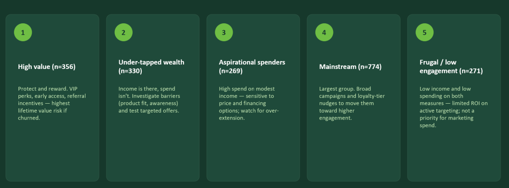
For segmentation, KMeans was applied to remuneration and spending (deliberately left unscaled, since both variables share a comparable, interpretable numeric range), with k selected only where the elbow method and sklearn.metrics.silhouette_score agreed, rather than from either metric alone. Cluster centroids were plotted on remuneration-spending axes on consistent, shared scales alongside elbow and silhouette plots across a range of k values, so the choice of k=5 is independently checkable rather than simply asserted. A summary table of cluster sizes and means was included in the presentation alongside the scatterplot, to simplify cluster definitions in assessing the commercial viability of any targeting strategy. For each cluster, a specific marketing strategy was recommended.

Fig 2: Clusters and Summary Table

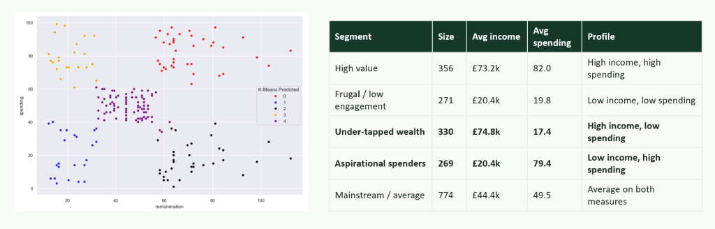
Fig 3: Recommended Marketing Strategies

STEP 5: Text Analysis

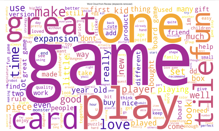
For text analysis, NLTK and TextBlob were used for tokenisation, stopword removal, word-frequency counts and polarity/subjectivity scoring, applied separately to the review and summary fields after observing early on that the two differ materially in descriptive content. A word cloud (generated after stopword removal, so the result was not dominated by common connecting words) was used to visualise the most frequent terms in the reviews. Word frequency on its own is a weak measure of sentiment, since a word appearing often says nothing about whether it is used positively or negatively; the word cloud was therefore treated as an illustrative, exploratory step rather than quantitative evidence. Polarity and subjectivity were each plotted as histograms rather than summarised as single averages, because the distribution shape, including a spike at zero polarity and a right tail toward +1, reveals a measurement artefact (short or neutral reviews TextBlob cannot meaningfully score) that a single mean would conceal entirely.

Fig 4: Text Analysis

Summary

Three patterns stand out. First, loyalty points are driven overwhelmingly by spending score and remuneration (combined R-squared=0.842, test R-squared=0.829), with age contributing only marginally; the pruned tree independently confirms this, splitting first on spending score and thereafter exclusively on remuneration. Second, customers form five stable, commercially distinct segments based on remuneration and spending, ranging from a high-value group worth protecting to a frugal, lowengagement group unlikely to repay active targeting. Third, negative reviews are not random noise: independent reviews converge unprompted on a specific, recurring complaint about instruction and assembly difficulty, a stronger and more actionable signal than aggregate sentiment scores alone would suggest.

To view the Pythonscript, click here. To view the R script, click here. To view the presentation, click here.